
We now have results for most seats in the South Australian lower house, with the final distributions of preferences due this week. We also know the broad strokes of what happened – Labor polled less than 40% of the vote, yet managed to win almost three quarters of the seats. So how did that happen? For this vote I want to explore the shape of the vote – how well was Labor’s vote distributed, and does that explain their ability to win such a large number of seats on such a low vote. I’ll also look at the two-candidate-preferred votes as well.
I have been reading some very old psephological work from the 1970s recently, and a tool used often by analysts like Malcolm Mackerras was a histogram, often showing the distribution of swings. This is a special kind of bar graph where each column lists how many cases fit in that range or bucket.
For this post I am using primary vote totals as of Saturday afternoon, and two-candidate-preferred figures as of Monday morning. Neither is final, but they are close enough to give us a sense of the shape.
Let’s start with the primary vote.
This chart shows the distribution of primary votes for the three largest parties. Seats are coloured based on who won that seat.
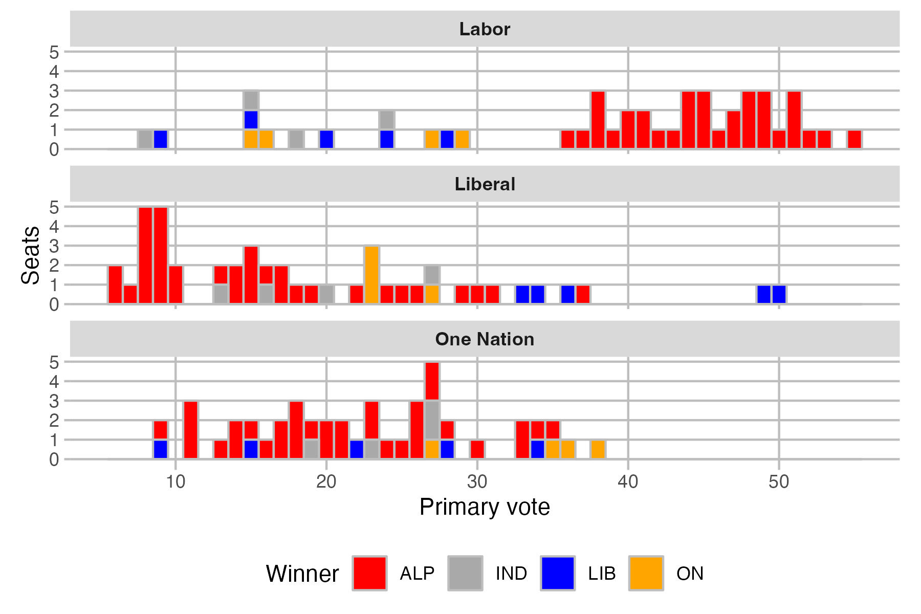
The Labor part of the graph is stark – there is not a single seat where Labor polled between 29% and 35% of the primary vote. And every seat over 35% they have won. The only seat below that line where they have come close is Heysen, where a high Greens vote means Labor could win on a lower vote. We will get to the 2CP margins later, but Labor is currently on 49.5% in Heysen and their next best seats are Hammond on 45.2% and Ngaduri and Bragg in the low 40s. There just wasn’t many close losses for Labor.
So part of the story for Labor in terms of their vote efficiency is that when they lost, they lost big. But they also didn’t rack up huge piles of votes where they weren’t needed. Labor’s primary vote only exceeded 50% in six seats.
If you look just at the 34 seats Labor has won, their primary vote averaged at 45.2% and their 2CP vote averaged at 62.2%. They managed a primary vote that generally was enough to win modestly, and also did quite well on preference flows to push a vote in the 40s into the 60s.
Normally you would expect a party winning comfortably to also poll respectably in their losing seats, thus adding to their overall vote total. But Labor is now at a point where they poll very poorly in places where they aren’t winning. And this has a geographic component – most of those Labor wins were in Adelaide, and just one non-Labor win was in Adelaide.
The Liberal and One Nation charts are also somewhat interesting, in particular showing how many seats had very low Liberal primary votes. I think this is something we will have to factor in when we consider how much Liberal preferences flowed to One Nation – in some seats the Liberal vote collapsed so far that they don’t make up a dominant part of the pool of preferences.
This next chart shows the range of primary vote swings for Labor, Liberal and the Greens – there’s not much to show for One Nation, since they only ran in a handful of seats in 2022.
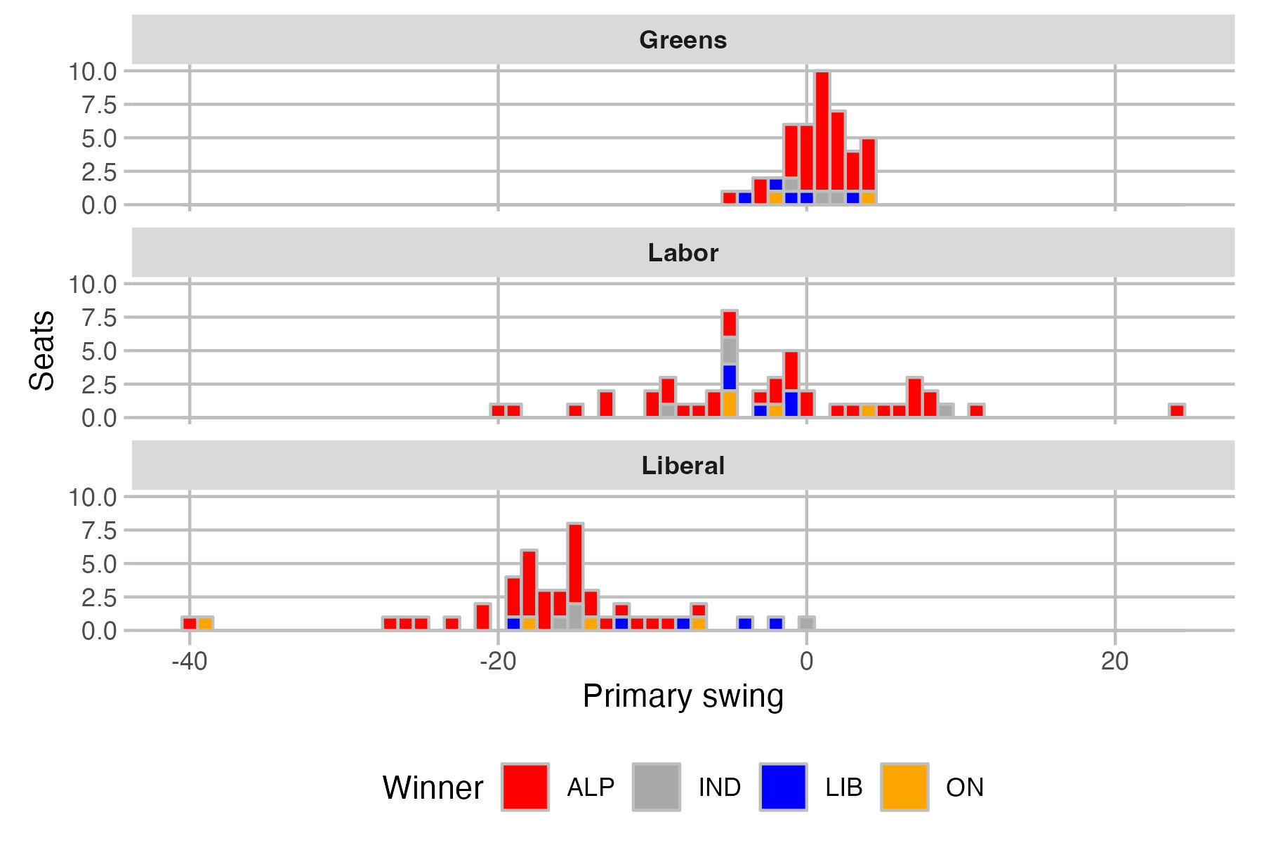
The Greens swings are very tight, with a majority showing a small swing. This isn’t surprising since the Greens vote tends to be a bit lower so doesn’t have as much room to move.
The swings were far from uniform for Labor – they gained a 24.6% swing in Waite and lost almost 20% in Light.
The Liberal swings were huge but there is clearly a focus point – 22 seats had the Liberal candidate suffer a swing of 15-19%. That’s almost half of the state.
Now let’s look at two-candidate-preferred figures. I am using William Bowe’s figures on his website, although I am using the current Labor-Liberal count in Heysen, not an estimated Greens-Liberal count.
At the time of writing, there are 26 Labor-One Nation contests, 13 Labor-Liberal contests, four Liberal-One Nation contests, two independent-One Nation contests, one independent-Labor contest and one independent-Liberal contest.
I will grapple with what a post-election pendulum will look like on another day, likely when we have the final distributions of preferences, but I suspect part of it will be presenting it as Labor vs Liberal/One Nation. If you look at things that way, it covers all but eight seats. Effectively you can see Labor as having two main opponents, with those parties having different strengths in different areas.
I also expect we will be doing a table showing not just the main margin, but an estimated alternative margin (for example, Labor-One Nation and Labor-Liberal) and the margin on the 3CP to change the top two.
So this chart is similar to the first primary vote chart, but it shows the two-candidate-preferred vote in every seat for each party that made that count (so each seat is shown twice). It is easy to identify whether that party won the seat (is their 2CP over 50%?) so instead I have colour-coded based on who the opposing party is.
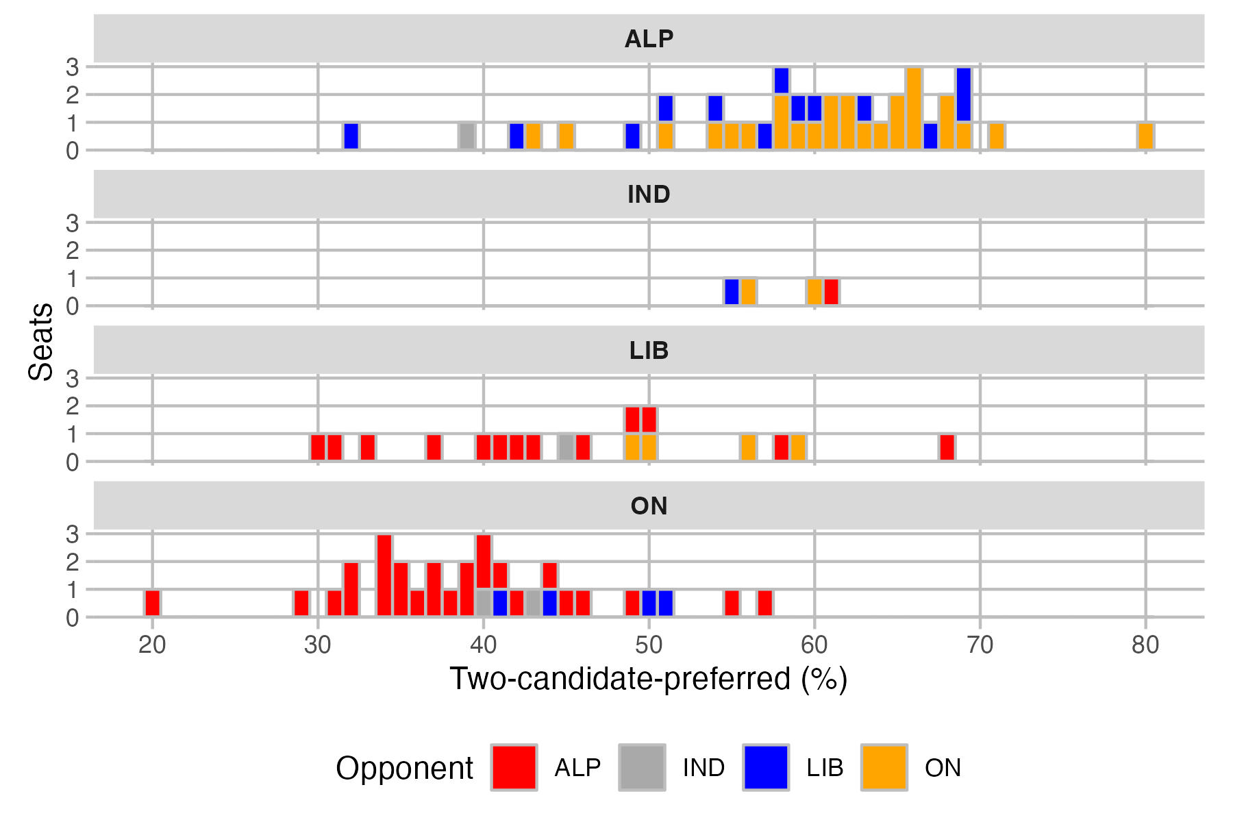
Again we see that Labor doesn’t have many super-safe seats on huge margins (one on 79.6%, another on 70.9%.
This also can perform some of the same functions as a pendulum. We can see that if there was a 10% swing from Labor to Liberal/One Nation, Labor would lose eight seats to One Nation and four to the Liberal Party. One Nation dominated the Liberal Party in a lot of places where the combined right-wing vote wasn’t enough to win.
Finally, this chart compares 2CP margins before the election (2022 results redistributed for 2026 boundaries) to the results of this election.
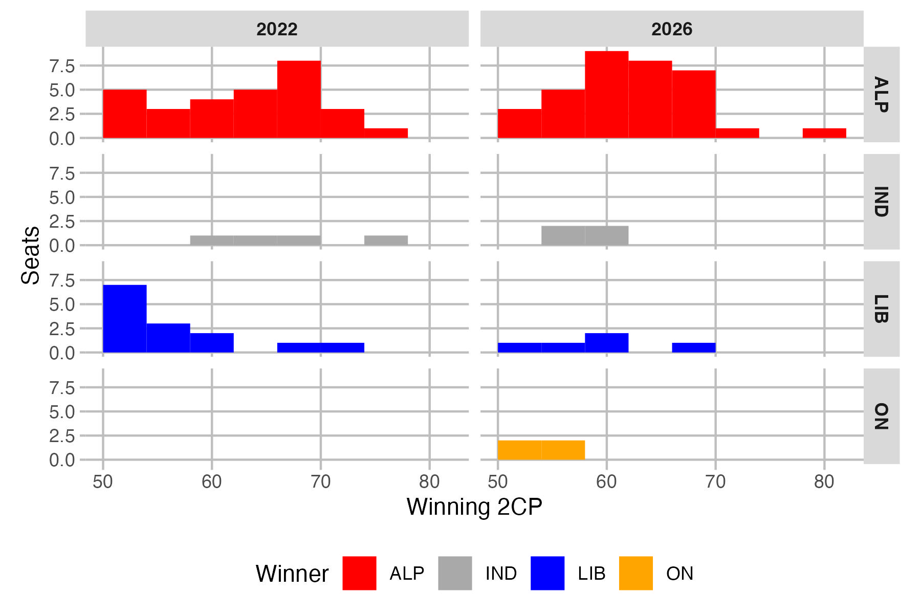
The number of conventional marginal seats has shrunk tremendously. On the old boundaries, there were five Labor seats and seven Liberal seats on margins under 4%, with a further six on margins of 4-8%. Now there are just six seats on margins under 4%, with another ten on margins of 4-8%.
The Liberal Party was particularly reliant on marginal seats prior to this election, so it is not surprising that they would lose so many seats.
Sometimes you would expect to see a party that has gained seats to have simply increased its vote everywhere, and thus see seats move to the right on this chart. But Labor hasn’t really gained super-safe seats. They had three seats with margins of 70% or more, and now there are two. They have particularly gained seats in the 8-16% range. Again, this points to remarkable vote efficiency for Labor. They are gaining election-winning numbers in most seats without getting much more than they need.
So let’s go back to the original question – why did Labor win such a huge number of seats? I don’t think much of the story is explained by preferences. There were just four come-from-behind wins. Labor was overtaken by the independent in Kavel and One Nation in Hammond, Labor overtook the Liberal in Morphett and the independent overtook the Liberal (and possibly Labor) in Finniss.
If this was a first-past-the-post election and there was no change in how people voted, Labor would have won 35 seats, the Liberal Party seven, One Nation three and independent two. It’s not much different to the result we will get.
The story here is that Labor was the biggest party, and were fairly efficient at distributing their votes in seats they won and not in any others. In general, they started the count well out in front of their conservative rival (be that One Nation or Liberal) and then gained enough preferences to maintain that lead.
And how solid was that win? It was fairly solid, with Labor not particularly reliant on close marginal seat wins. If there was a uniform swing of 8.7% on the 2CP from Labor to either of the two big right-wing parties, Labor would lose eleven seats. This would leave them with just 23 seats, one short of a majority.
A 10% 2CP swing would be quite big, but I think such a swing would put the state roughly on a 50-50 balance. Across the 39 seats where Labor is in the top two against Liberal or One Nation, the Labor 2CP averages to 59.7%. Once you factor in the very conservative seats where Labor didn’t make the top two, I suspect a Labor 2PP of about 58-59% would be about right. So if a swing of 8.7% leaves Labor just short of a majority, that sounds to be roughly balanced between the left and right.

An adjustment is needed to this sentence: “Labor was overtaken by the independent in Kavel and One Nation in Hammond, Labor overtook the Liberal in Morphett and the independent overtook the Liberal (and possibly Labor) in Finniss.” I just looked at the ECSA site (10.30am, 2nd April) and the final Primary vote result in Hammond had One Nation on 6,442 votes and Labor on 6,353, whereas in Morphett it was Labor 8.052 and Liberal 7,857 – so that it seems in only two seats did the candidate who lead on first preferences not end up winning. Also, if we’d had first past the post, Labor would have won 35 seats, not 34.
This was correct when the data was collected. I will do a final sum-up of those statistics when results are final.